When comparing a sample before and after some operation has been done to the sample, we use the Paired T Test. In this example, we’re comparing diameters of a group of parts both before and after a grind operation. We want to know if the grind operation, which is supposed to just remove surface irregularities, is actually changing the diameter of the parts.
To create a template for our data, click the “Compare data sets” button, and select “Paired T Test”. You will see the following dialog:
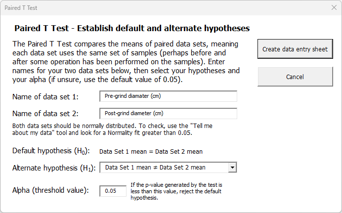
First, we need to name our data sets. We’ll name data set 1 — the part measurements taken before the grind operation — as “Pre-grind diameter (cm)” and data set 2 will be for the measurements of those same parts taken after the grind operation. We’ll call that “Post-grind diameter (cm)”.
Then we need to select our hypotheses. The default hypothesis (written as H0 and referred to as the “null-hypothesis” or “h-naught”) is that mean diameter of the samples taken “pre-grind” is statistically the same as the mean diameter of those same samples “post-grind”. Of course, we also must have an alternate hypothesis (written as H1, sometimes called “h-one”). The alternate hypothesis can take one of three forms:
- The means are not the same (this is the most general form, and the default setting in the dialog)
- The mean of Data Set 1 is greater than the mean of Data Set 2
- The mean of Data Set 1 is less than the mean of Data Set 2
In this case, we’re just interested in knowing of the before and after diameters are different, so we’ll leave the alternate hypothesis as:
“Data Set 1 mean ≠ Data Set 2 mean”.
Then we need to choose our alpha value for the hypothesis test. In traditional hypothesis testing, we begin by assuming that the characteristic we’re assessing (diameter in this example) is statistically the same for both data sets (the default hypothesis stated above). We won’t be willing to reject that default hypothesis unless we reach a certain confidence level that the means of the two data sets really are different. The key question you need to answer is: how confident do we need to be to reject the default hypothesis and accept the alternate hypothesis? That’s where alpha comes in. If we want to be 95% confident that the data sets have different means before rejecting the default hypothesis, then we need to set alpha to 0.05 (the default setting in the dialog). If we want to be even more confident (say, 99%), then we should set alpha to 0.01. In this case, let’s leave alpha at 0.05, then click the “Create data entry sheet”.
On the sheet, we enter the names of the samples and the measurements for each sample both before the grind operation and after. With all the data entered, we see the results:
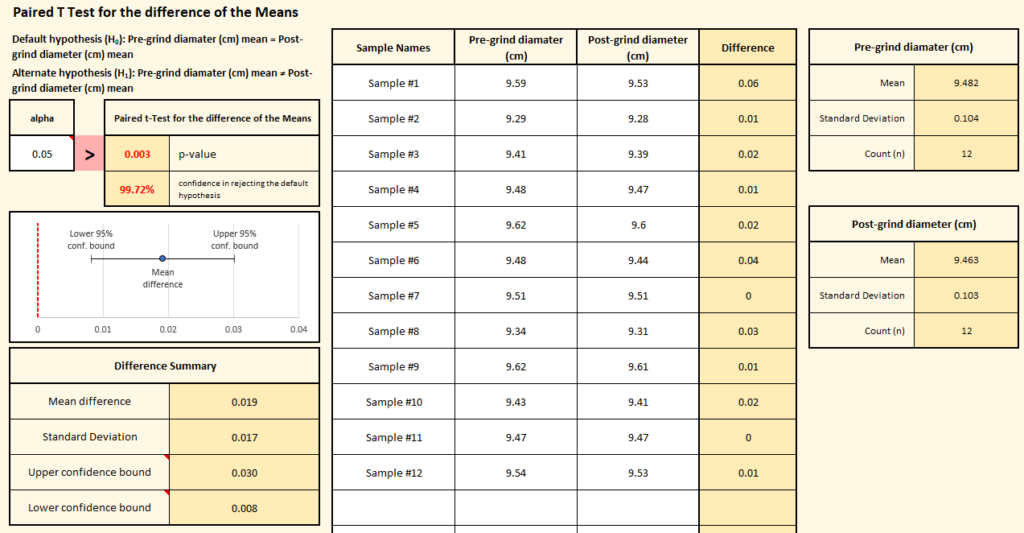
The first thing we notice is that the p-value (highlighted in red, in the upper left corner) is 0.003, which is below our alpha value. By setting our alpha at 0.05, we wanted to be 95% sure that the means of the two data sets really were different before we’d accept the alternate hypothesis. In this case, we’re 99.72% confident that the pre and post-grind means are different, so we must conclude that the grind operation is changing the diameter of the parts.
This is further illustrated in the graph. The average difference in the diameter between pre and post-grind is 0.019 (the blue dot), and the 95% confidence interval for that measurement does not include zero — which means that we’re very confident that the true difference is not zero (if the difference were zero, then the diameters would be the same pre and post-grind).