We use the F Test to compare the standard deviations of two data sets. We begin by assuming that the standard deviations are statistically the same for both data sets. This doesn’t mean that the standard deviations of the two sample data sets we’re looking at must be exactly the same, but rather that they are close enough to each other that the difference represents expected variation and is not statistically significant.
So, our default hypothesis (written as H0, and referred to as the “null-hypothesis” or “h-naught”) is that standard deviations are statistically the same. Of course, we also must have an alternate hypothesis (written as H1, sometimes called “h-one”). The alternate hypothesis can take one of three forms:
- The standard deviations are not the same (this is the most general form, and the default)
- The standard deviations of Data Set 1 is greater than the standard deviation of Data Set 2
- The standard deviation of Data Set 1 is less than the standard deviation of Data Set 2
Let’s look at a specific example to illustrate how this works. A software sales company has two offices (one in Springfield and one in Fairview) that each complete a series of standard work steps to close out completed customer sales. They have found that the time required to complete the work varies, and the Sales Manager wants to determine if one office is more consistent than the other. The manager gathers historical data: for the previous month, they find 17 completed requests processed by the Springfield office and 15 completed requests processed in Fairview.
To run the analysis, the Sales Manager starts by clicking the “Compare data sets” button on the SuperEasyStats ribbon and selects “F Test” from the menu of options. They then see the following dialog box:
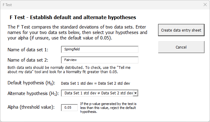
Notice that the default hypothesis is fixed. We always assume that the standard deviations are the same unless proven otherwise. Now the Sales Manager must choose the alternate hypothesis. They have no particular reason to think that one office has a larger or smaller standard deviation than the other, all they are really trying to determine is if the standard deviations are different. Thus, for their alternate hypothesis they select the default option: that the standard deviation of Data Set 1 (“Springfield”) does not equal that of Data Set 2 (“Fairview”).
They won’t be willing to reject the default hypothesis unless they reach a certain confidence level that the standard deviations really are different. The key question they need to answer is: how confident do they need to be?
That’s where alpha comes in. Alpha is a decision rule for rejecting the default hypothesis. If the Sales Manager wants to be 95% confident that the data sets have different standard deviations before rejecting H0, then they need to set alpha to 0.05 (the default value). But if they wanted to be even more confident (say, 99%), they would need to set the alpha to 0.01. In this case the Sales Manager just needs to be 95% sure that the standard deviations are different before accepting that as the case, so they leave the alpha value at 0.05 (the default setting).
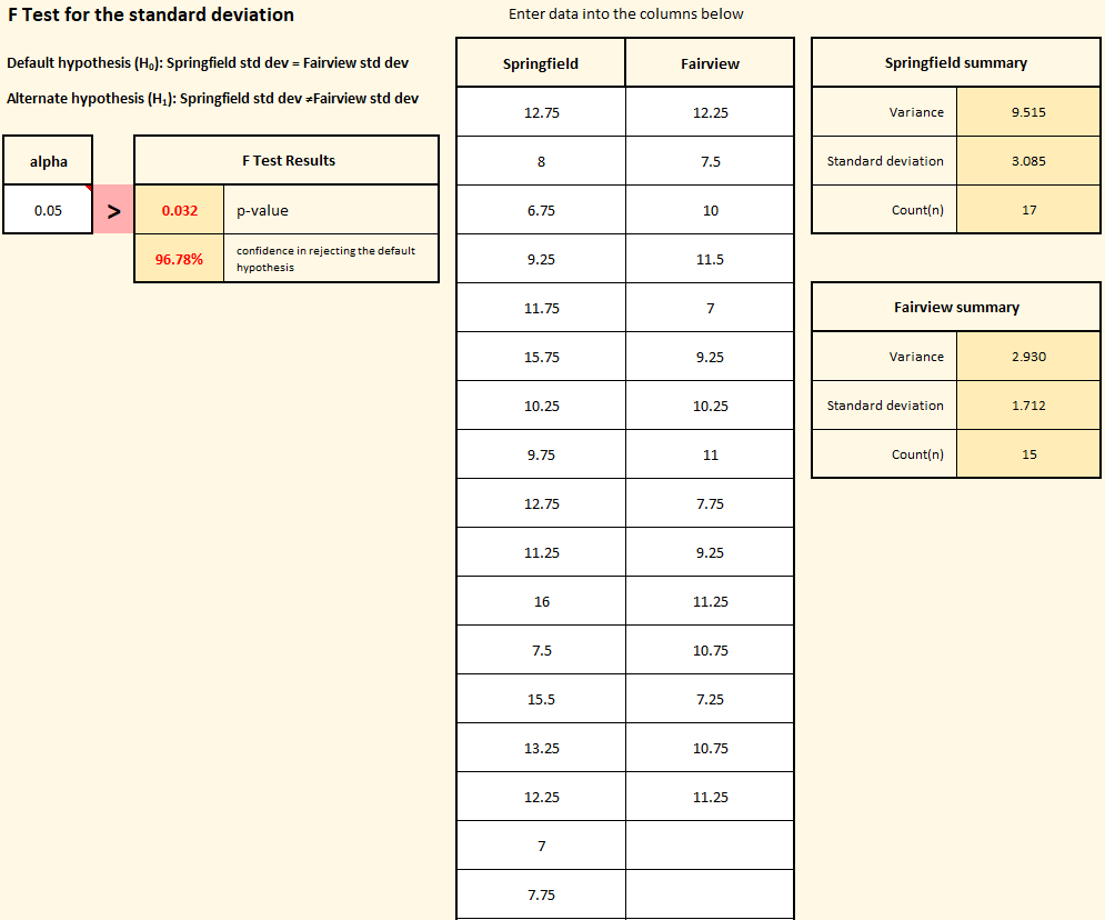
Once the hypotheses are selected and the alpha is set, the manager clicks the “Create data entry sheet” button. On the data entry sheet, they enter the historical data they had previously collected from Springfield and Fairview and paste it into the template. Below you can see the data entry sheet as filled in by the Sales Manager.
In the upper left corner, the hypotheses are shown. The previously chosen alpha value is displayed below that. In the center are columns where the Sales Manager entered the raw data. To the right of those columns are summary boxes showing the variance and standard deviation of each data set.
The key result is the p-value shown in the box labeled “F Test Results”. Notice that the p-value is 0.032. Since that is less than the Sales Manager’s chosen alpha value (0.05), they have met their threshold. They can be 96.78% certain that the alternate hypothesis is true, and remember, the alternate hypothesis is that the standard deviations between the offices are truly different.