The “Category data” button allows you to test for statistically significant correlations in categorical data. The following two examples illustrate how this works.
Example 1

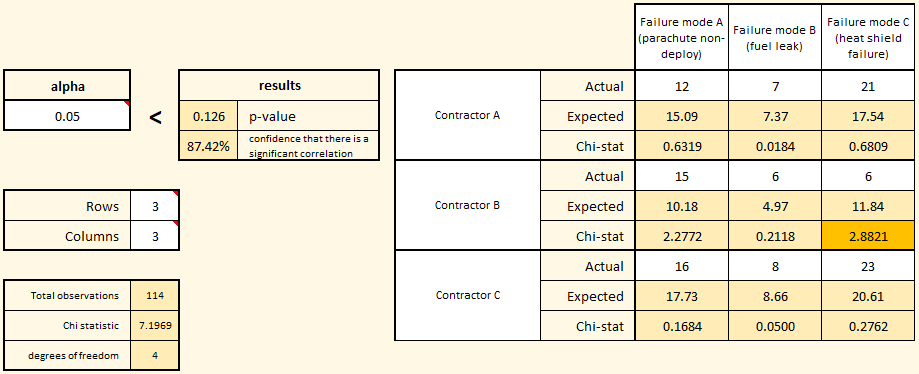
In the example on the right, three contractors have been hired to supply reusable orbital rockets. There are three problem areas of particular interest: parachute failures, fuel tank failures, and heat shield failures. Because we have three contractors and three failure modes, we select three rows and three columns for our matrix.
Each contractor launches an equal number of test rockets and counts the number of failures of each type. Our default hypothesis (H0, or h-naught) is that the failure type is independent of contractor. In this example, we want to be 95% certain that there is a correlation between failure type and contractor before we reject our default hypothesis and accept the alternative hypothesis (H1) that there is a statistically significant correlation. Because we want 95% confidence, we set our alpha value to 0.05.
As you enter the actual failure numbers into the matrix, the software will automatically calculate an expected number of failures by contractor and type. Once all of the actuals are entered, we see that the calculated p-value is 0.126, which is greater than our chosen alpha value. Based on the decision rule we established before the experiment, we should not conclude that there is a significant correlation between contractor and failure mode.
Note the highlighted Chi-stat in the matrix for Contractor B’s failure mode C (heat shield failure). That highlight simply shows you the largest deviation between the expected number of failures (assuming no correlation) and the actual number of failures that were observed. Based on the total number of heat shield failures across all contractors, and the total number of failures of all types produced by Contractor B, you would expect Contractor B to produce between 11 and 12 heat shield failures, but they only produced 6. So, while the actual number is less than what was expected, it doesn’t deviate enough to reach statistical significance.
Example 2
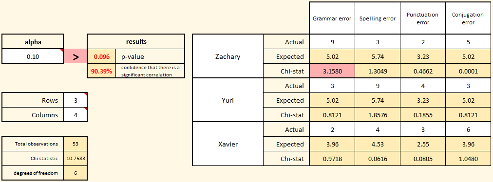
 In this second example, we are tracking the types of errors produced by three translators working in the communications department. Each translator was given the same document and the number and type of each error were counted. Because there are three translators and four error types, we change the size of the matrix to have three rows and four columns.
Notice that in this example, the alpha value was changed from 0.05 to 0.1. Remember, alpha is your decision rule. If the calculated p-value is lower than your chosen alpha, then you should reject the default hypothesis that there is no correlation between the translator and type of error. In this case, the manager of the communications department decided ahead of time that being 90% confident of a correlation would be strong enough evidence to initiate a root-cause investigation of the differences.
The actual errors by translator were entered into the matrix, and the result is a p-value of 0.096, which is lower than the chosen alpha value. In this case, based on the established decision rule (alpha), the default hypothesis (H0) should be rejected and the alternative hypothesis (that there is a correlation between error type and translator) should be accepted.
Note that the cell in the matrix with the largest Chi-stat (meaning the most unexpected deviation between actual and expected values) is highlighted (this time in red because the overall result is statistically significant). Note that the highlighted cell in the matrix may not be the only cause of the low p-value. There may be other deviations worth investigating as well. Look for cells with higher Chi-stats as you do your root-cause investigation. The highlighted cell is a good place to start.
Copyright 2020 David Margil
