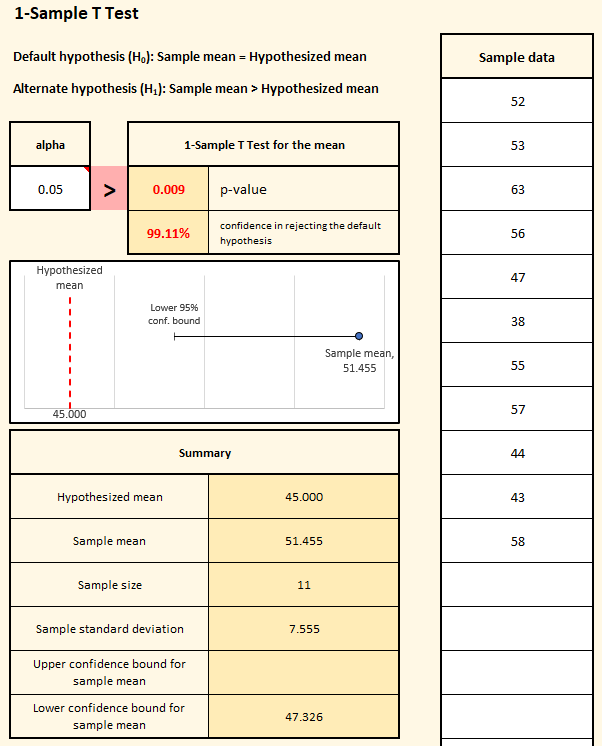
The 1-sample T Test compares the mean of a sample to a hypothesized (or known historical) mean value. The sample data should be normally distributed (you can use “Tell me about my data” to confirm normality).
As an example, a consulting company’s accounts receivable department suspects that one of it’s largest clients is taking longer to pay invoices than it used to. If that is true, the accounts receivable manager will need to call the client and ask them to speed up payment. But the manager wants to be sure before making that call. They don’t have records of how long previous payments took, but they believe that, on average, the client used to pay in 45 days. To see if payments really are taking longer, the manager starts keeping detailed records of how long new invoices are taking to be paid. After six months, they have data for 11 invoices, and they decide to use a 1-sample T Test to see if the average time for those invoices is statistically different from the hypothesized mean of 45 days. First they confirm that the sample data is normally distributed. After confirming that, they click the “Compare data sets” button on the SuperEasyStats ribbon and select “1-Sample T Test” from the menu of options. They then fill in the following dialog box:

In the “Value of hypothesized mean” field, they enter 45, because the manager believes that’s the historical average for this customer.
The default hypothesis is that the Sample mean is equal to the hypothesized mean of 45 days.
The alternate hypothesis can take one of three forms:
- The means are not the same (this is the most general form, and the default option in the dialog box)
- The mean of the sample is greater than the hypothesis mean
- The mean of the sample is less than the hypothesis mean
In this case the manager strongly suspect that client is take longer than the previous average of 45 days, so they select “Sample mean > Hypothesized mean”.
They then need to choose the Alpha value for the test. They won’t be willing to reject the default hypothesis unless they reach a certain confidence level that the sample mean really is greater than the hold, hypothesized mean. The key question they need to answer is: how confident do they need to be?
That’s where alpha comes in. Alpha is a decision rule for rejecting the default hypothesis. If the accounts receivable manager wants to be 95% confident that the new average time to pay is greater than before, then they need to set alpha to 0.05 (the default value). But if they wanted to be even more confident (say, 99%), they would need to set the alpha to 0.01. In this case the manager decides that 95% is good enough, so they leave the Alpha at 0.05 (the default setting for the dialog). Then they click “Create data entry sheet”.
On the data entry sheet the manager enters the days to pay for the 11 invoices in the sample:

