 The Variable Data Capability function can be used to understand important quality metrics about your process. Let’s look at an example.
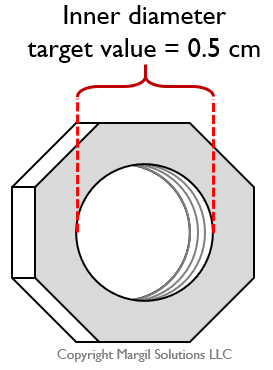
A parts manufacturer produces bolts for a customer. The customer requirement is for the bolts to have an inner diameter of 0.5 cm +/- 0.01 cm. Recently they have been getting complaints that too many bolts are falling out of spec and are unusable.
They decide to better understand their process and so they set up a sampling plan. There are three shifts, and each shift they will randomly pull 20 bolts and measure their inner diameters. The data is shown at left, entered onto a plain Excel sheet.
Next, they select the “Variable data capability” button on the SuperEasyStats ribbon in Excel and select just the cells with the data (not the titles or the sample numbers), as shown below:

In addition to selecting the data, you can optionally fill in a chart title, and one or both of the upper and lower specification limits. In this case, because the target diameter is 0.5 cm +/- 0.01 cm, they entered 0.51 for the upper specification limit, and 0.49 for the lower. Once the dialog is filled in, click the “Calculate capability and histogram” button. You will see the following chart, and the dialog box will remain, allowing you to adjust the graph as needed:
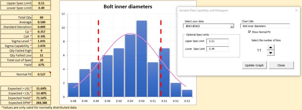
Here the “number of bins” (vertical columns on the graph) has been adjusted from the default (20) to 11. The dotted red lines represent the locations of the upper and lower specification limits. Once the graph is adjusted to your preference, you can click “Close”.
 Next to the graph are a number of important statistics:
-
-
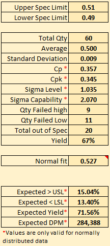
- Upper and lower specs are the limits you entered when you created the graph.
- Total Qty is the number of individual data points in the sample used to create this graph.
- Average and Standard Deviation of the data in the sample. In this case, the average inner diameter is right where the customer wants it, at 0.50 cm.
- Cp and Cpk are key capability measures.
- Cp is the ratio of the width of the spec limits to the width of the process (defined as the average, plus and minus 3 standard deviations). If Cp is less than 1, then the process variation too wide to fit within spec. Generally, a Cp of 1.5 is considered quite good. The Cp calculation does not take into account where the process average is relative to the specification limits. Note that both an upper and lower spec limit are required in order to calculate Cp.
- Cpk is a measure of how close the process average is to the nearest specification limit. The smaller the number, the closer the process average is to one of the spec limits, and therefore more process output is falling out of spec. Ideally, the process average should be centered between the specification limits, which helps minimize Cpk. However, even when centered (as this process is), if the standard deviation is too large, parts will still be out of specification. Increasing Cpk involves moving the process average to the center of the specification limits, and decreasing the overall variation in the process. A Cpk of 1.5 is considered very good. Note that at least one spec limit must be provided to calculate Cpk.
- Sigma Level Is a measure of how many standard deviations can fit between the mean of the distribution and the nearest specification limit. There must be at least one specification limit to calculate Sigma Level.
- Sigma Capability is a function of defects per million opportunities (dpmo) and is useful for comparing quality levels of products that different levels of complexity. Traditionally, a true 6 sigma capability process would have 0.002 defects per million. However over time processes exhibit variation and it has become somewhat standard to assume that processes can drift up to 1.5 standard deviations from the mean. Thus a 6 sigma capable process will behave like 4.5 sigma process (taking into account the expected drift) will actually exhibit 3.4 defects per million.
- Sigma capability of 2 equates to 308,538 dpmo
- Sigma capability of 3 equates to 66,807 dpmo
- Sigma capability of 4 equates to 6,210 dpmo
- Sigma capability of 5 equates to 233 dpmo
- Sigma capability of 6 equates to 3.4 dpmo
- Qty failed high and Qty failed low show how many items in this sample were above or below the spec limits. Note that at least one spec limit must be provided to calculate the quantity failed metrics.
- Yield shows the percentage of items in this sample that were within the specification limits. Note that at least one spec limit must be provided in order to calculate yield.
- Normal fit is based on a statistical test* designed to determine if the data in the sample fits the Normal distribution. This is important for multiple reasons, but in this context, it is critical to interpreting the Cp and Cpk results, both of which are based on the assumption that the data is Normally distributed. Generally speaking, if the likelihood of normality falls below 5%, you should assume the data is not normally distributed, and therefore the Cp and Cpk values should not be used.
-
The following shows what you can expect from your process if it keeps exhibiting the same level of quality as your sample and it follows a Normal distribution:
-
-
- Expected > USL shows the percent of the process output you should expect to exceed the upper specification limit, based on this sample.
- Expected < LSL shows the percent of the process output you should expect to fall below the lower specification limit, based on this sample.
- Expected Yield shows the percent of the process output you should expect fall inside the specification limits, based on this sample.
- Expected DPM shows how many defects per million you should expect, based on this sample.
-
* SuperEasyStats uses the Anderson-Darling test to assess Normality.